|
|
| Copyright © Klaus Piontzik | ||
| German Version |
| The American physicist James Bjorken found
in 1969 that there appears to be a logarithmic scale invariance in
the frequency distributions of elementary particles depending on
their rest mass (Bjorken, Feinmann).
In 1987, Hartmut Müller expanded the discoveries for all known particles, nuclei and atoms as well as asteroids, moons, planets and stars. The global scaling theory is intended to describe structuring phenomena of matter in the universe. Global Scaling Definition: The basis of the theory can be summarized as follows: If any quantitative properties of natural systems, i.e. frequencies, sizes, masses, lifespan, etc. of elements, atoms, molecules, cell organelles, cells, organs, organisms, populations, moons, planets, stars or galaxies are arranged on a logarithmic scale, then these values ??are not evenly distributed but cluster in certain zones while other zones almost remain empty. A so-called standard measure is used to ensure appropriate scaling. For years, the global scaling construct has been the background for fraud and the marketing of various charlatan products and questionable services such as lottery predictions. The inventor Hartmut Müller was sentenced to several years in prison for fraud. Global Scaling was also classified as a pseudo-scientific-esoteric conglomerate. Psiram and other sites on the Internet present Global Scaling as pseudo-science, but all of these sites fail to provide any evidence. Here is the mathematical proof that the choice of standard in global scaling is purely arbitrary and therefore the global scaling theory is at least superfluous or that global scaling represents an arbitrary speculative construct. |
| There are n
alues ??given, namely: w0,
w1, w2,
... wk, ... wn
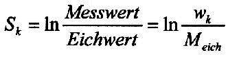
There are calibration values Meich in Global Scaling that are based on the physical quantities of the proton Scaling in Golbal Scaling is defined by the following equation |
| 7.7.1 - Equation: |
|
| Due to the laws of logarithms: |
|
| According to Equation 7.4.5: |
|
| This is how you can write: |
|
| Inserting the term for y: |
|
| According to Equation 7.4.4: |
|
| Overall this results in: | |
| 7.7.2 - Equation: |
|
| Inserting all terms gives: | |
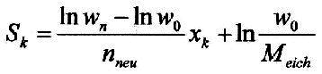
| 7.7.3 - Equation: |
|
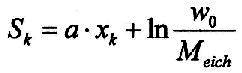
If the standard measure is set equal to 1 (Meich = 1) the equation 7.4.5 simply arises: Sk = yk = axk+b That means: 1) There is a functional connection between the e-function finding procedure described here and global scaling 2) The procedure described here provides a form of scaling that is fundamental in nature, while global scaling represents a more derived quantity because a certain standard is used there. This can be seen from the fact that in Equation 7.7.2 the standard measure only appears in the additive component of the straight line equation. If all values ??are given, this term simply represents an additive constant. However, the actual scaling process takes place in the first term. You can also represent it like this: The additive constant gets a new name: 7.7.4 - Definition: |
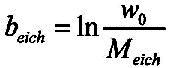
Then the scaling function can also be represented like this: 7.7.5 - Equation: |
![]()
|
This means that we have a straight line equation in front of us.
The slope of the line is represented by the first term ax.
The additive constant b only shifts this line vertically, i.e. along the y-axis.
3) The procedure described here is an equivalent to global scaling. This confirms global scaling once again with regard to the logarithmic structure of the universe (see also chapter 8). However, equations 7.7.2 and 7.7.4 show that the choice of standard is arbitrary. Instead of the proton sizes in global scaling, any other size such as the electron can be used.
Mathematically it is much more natural to set the gauge equal to 1
(Meich = 1) .
The planetary orbits serve as an example here. The table contains
the original numbering (old), as well as the approximate numbering
from the linearization and the calculated numbering.
|
| Planet | Nr | Distance | Nr | xk | a·xk | Global Scaling |
| old | [AE] | approximated | calculates | a·xk+beich | ||
Mercury |
0 |
0,3871 |
0 |
0 |
0 |
60,88009872 |
Venus |
1 |
0,723 |
1,3 |
1,182 |
0,624726165 |
61,50482488 |
Earth |
2 |
1 |
1,9 |
1,796 |
0,949072221 |
61,82917094 |
Mars |
3 |
1,524 |
2,6 |
2,593 |
1,370410679 |
62,25050940 |
Asteroids |
4 |
2,7 |
3,75 |
3,675 |
1,942323994 |
62,82242271 |
Jupiter |
5 |
5,203 |
5 |
4,916 |
2,598307604 |
63,47840632 |
Saturn |
6 |
9,582 |
6,1 |
6,071 |
3,208958560 |
64,08905728 |
Uranus |
7 |
19,201 |
7,5 |
7,386 |
3,904034582 |
64,78413330 |
Neptune |
8 |
30,047 |
8,25 |
8,233 |
4,351835044 |
65,23193376 |
Pluto |
9 |
39,482 |
8,75 |
8,750 |
4,624917093 |
65,50501581 |
| In Global Scaling, the natural wavelength of the proton
is given as a standard value of 2.103089 10-16
m This results in beich = 60.88.
The following applies to the planetary orbits: a = 0.52856 (see page 176)
The calculated numbering values xk
reflect the absolute harmonic relationships of a system and are completely independent of a standard..
Here in this chapter you can also replace ln with log in all equations. |
|
200 sides, 23 of them in color 154 pictures 38 tables Production und Publishing: ISBN 978-3-7357-3854-7 Price: 25 Euro |
![]()