|
|
| Copyright © Klaus Piontzik | ||
| German Version |
| Generally, you can put 11 elevant atmospheric layers together. The individual layers are sorted and numbered according to height. |
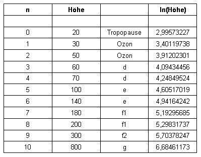
| Right in the table is the logarithm naturalis
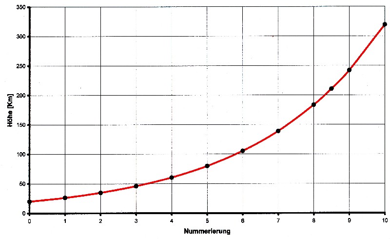
for the respective heights. The logarithm of height is represented as a function of numberin: |
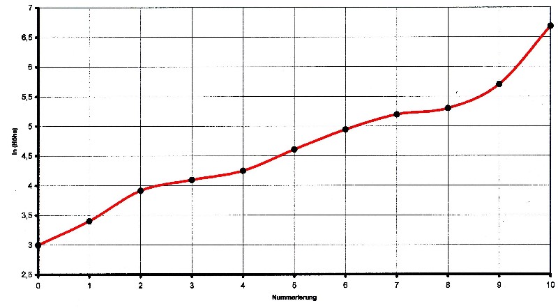
| Illustration 3.8.1 – logarithm of height |
| The function in illustration 3.8.1,
seems to be not very linear on first view ex-cept in few parts.
If you look but closer to the course so you can see a)Between the points 2 to 7 the slope is nearly constan b)Between points 1 and 2 as well as between points 2, 8 and 9 is the slope so large, there can still a point be inserted, to flatten the slope c)Between points 9 and 10 the slope so large that there still several points can be inserted. Therefore, point 10 is eliminated first d) Between point 7 and 8 the slope is so small that there the numbering can be used on a half, increasing so the slope The following table shows the layers that are corrected in the numbering arranged by height: |
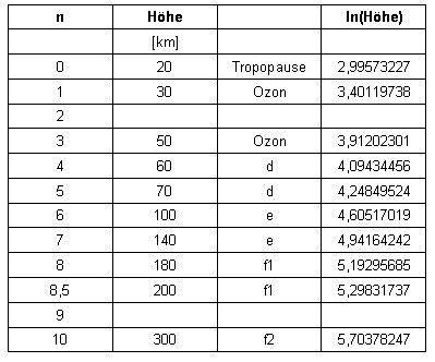
| The newly added layers at the numbers 2 and 9 are clear to see in the table. The corrected function looks like this: |
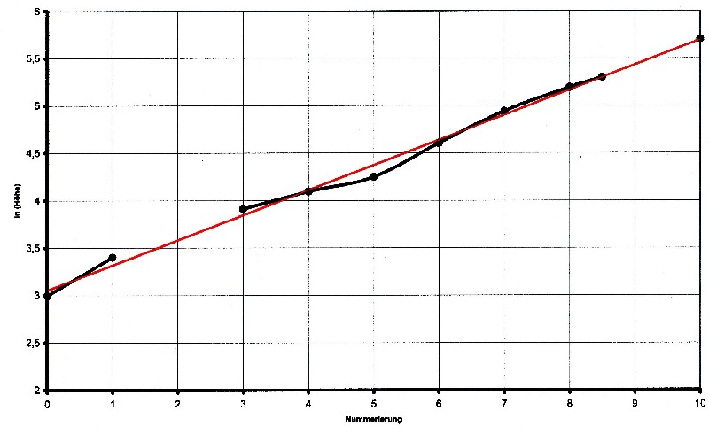
| Illustration 3.8.2 – logarithm of height |
| The red line in illustration 3.8.2 represents
a linear function that was obtained by linear regression from the corrected table.
Like is to see the layers values match well with the approximation function. It can be used here so a linear function for the atmospheric layers as a solution. The following applies to the additive constant: b = ln wMin = ln H0 = ln 20 = 2.995732 The following applies to the slope of the line: Δ y = ln wMax – ln wMin = ln 320 – ln 20 = 2.772588 Δ x = n = 10 a = Δ y/Δ x = 2.772588/10 = 0.277258 A linear function for the atmospheric layers can be used here as a solution approach. In general, the following applies to the straight line from Figure 3.8.2: y = ln(Höhe) = a·x + b The values ??found are inserted into the straight line equation: |
| It results: | ln(Hight) = 0.277 · x + 2.9957 |
| By rearranging you get: |
| 3.8.1 - Equation: | Hight = 20 · e0.277·x [Km] |
| Putting x = n then following function arises for equation 3.8.1: |
| Illustration 3.8.3 – Height as e-funktion |
| Equation 3.8.1 has all the properties that are necessary
to get as a solution function of Laplace's equation in consideration to 2.11.3. Thus the atmospheric layers represent a solution of Laplace's equation, specially for the radial part. In consequence the following sentence can be set up: |
| 3.8.2 - Theorem: | The atmospheric layers are an expression of an oscillation phenomenon |
| On the equation of 3.8.1 can be still made simplifications. Es gilt: 0.277 = 3.6-1 = 5/18 When all values are used: |
| 3.8.2 - Equation: | 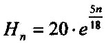 |
[Km] |
| It can be made to the following relation (see Theorem 5.1.5): rik= RE/5 · rik = inner core and RE = 6371 Km and it still applies: 5100 = RE– rik = 4/5 · RE = 4rik 5100 = 255 · 20 ==> 20 = 4/255·rik Then you can write for the atmospheric layers: |
| 3.8.3 - Equation: | 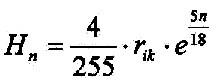 |
[Km] |
| Then you can continue to write for the atmospheric layers |
| 3.8.4 - Equation: | 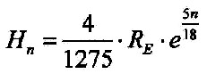 |
[Km] |
| The layers arranged by height and the calculated values result in the following table: |
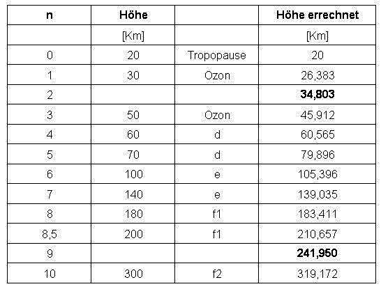
| The mean error of the calculated values for the layers is below 2 percent. In addition, even 2 layers arise |
|
200 sides, 23 of them in color 154 pictures 38 tables Production und Publishing: ISBN 978-3-7357-3854-7 Price: 25 Euro |
![]()